Developing an ML Program for Credit Card Fraud

Hello, today I decided to take a step away from the climate stuff because I’m having difficulty finding datasets that are accessible and useful. But I still wanted to present a project so I decided to look at Kaggle’s highest rated dataset and found this. In this post I’m going to talk about my strategies when confronting problems like this and talk about how I work through them and eventually come to a usable solution!

Note: I am following a similar structure to Aurélien Géron‘s Hands on Machine Learning with Scikit-Learn & TensorFlow.

Overview:

This project is a quick look into using classification ML algorithms to distinguish extreme outliers in a given dataset. Although this is an example with credit card transaction data to detect fraudulent activity there are ways this can be applied to climate based issues and solutions! Some examples are: looking for anomalous data in climate data, whether it’s from a bad sensor or just simple quality control in data; finding and recognizing extreme weather events that should be flagged as potentially dangerous; using it on building management systems to detect leaks or excess uses of energy in certain areas; the list goes on and on and there’s really no lack of potential use-cases where it can be applied.

This dataset is gathered from Kaggle, you can find it here. The dataset has 31 features: Time, Transaction Amount, Class (fraud: 1, not fraud: 0), and 28 hidden features (V1 – V28). Unfortunately, because of confidentiality issues the dataset cannot provide insight onto what the hidden V features are, but it is no matter, we can still develop a highly effective classification system.

Code:

I’m going to very quickly cover analysis of the data just to highlight its importance but not make this post too long. It’s always good to take a look at what the data looks like and what you’re dealing with. This will help give you some insights as to things you should focus on, and just make you more confident about how to interact with the dataset.

import pandas as pd
import numpy as np
import matplotlib.pyplot as plt

data = pd.read_csv('creditcard.csv')

# Here are the ways I take a first look at the dataset before anything else:

# general info:
print(len(data))
data.head()
data.info()

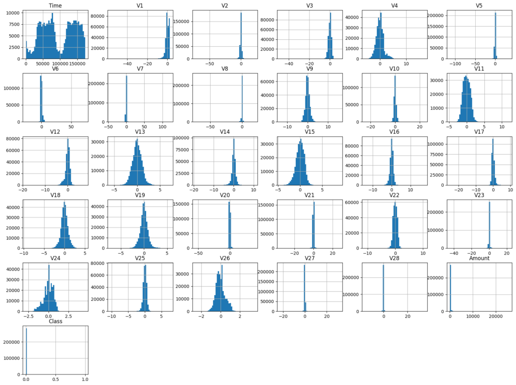
# plotting histograms and getting a visual sense of the data:
data.hist(bins = 50, figsize = (20,15))
plt.show()

In this project I also wanted to see what the ratio of fraudulent vs. non-fraudulent cases was. This will eventually help decide how we program our ML algorithm.

def percent_of_fraud_calc(data):
    fraud_no = len(data[data['Class'] == 1])
    not_fraud_no = len(data[data['Class'] == 0])
    percent_of_fraud = (fraud_no / not_fraud_no * 100)
    print('Number of Fraudulent transactions: ', fraud_no)
    print('Number of Non-Fraudulent transactions: ', not_fraud_no)
    print('Percent of Fraudulent transactions: ', percent_of_fraud, '%')

percent_of_fraud_calc(data)

* Number of Fraudulent transactions:  492
* Number of Non-Fraudulent transactions:  284315
* Percent of Fraudulent transactions:  0.17304750013189596 

This demonstrates a massive imbalance in our dataset which, if left as is, will result in a very skewed result which I’ll address later.

After getting a quick sense of the data and looking at the histograms we see that nothing looks too out of the ordinary. However, we do see that most of the data seems to fall between the -3 to +3 range (very roughly) except for the time, and amount. So we will want to scale those down. The reason for scaling data is because features that have a much bigger range will have more “influence” than those with a smaller range. You can think of it as having a panel of judges. If there are 10 judges, 9 of whom are allowed to use a rating scale from 1-10 and then one judge who has a scale from 1-100 you can imagine how if the 9 judges sees a performance and rates a 10 out of 10! and then the 1 judge says poo poo to that and gives it a 1 the average score is a 9.1; now let’s say they see a performance where the 9 judges rate it a 1, but the one judge rates it a 100, now the mean is a 10.9. You can see how this will effect the decision making in an ML algorithm. This is why we use scalers and this is an important step in the preprocessing of data!

from sklearn.preprocessing import StandardScaler

std_scaler = StandardScaler()

data['scaled_time'] = std_scaler.fit_transform(data['Time'].values.reshape(-1, 1))
data['scaled_amount'] = std_scaler.fit_transform(data['Amount'].values.reshape(-1, 1))

data.drop(['Time', 'Amount'], axis = 1, inplace=True)

data.head()

Great! Now before we do anything else we have to split up our data into the training set and the test set. Because this dataset is quite simple we don’t need to use a stratified sampling method. But it never hurts to do so. If you’re dealing with diverse populations or datasets it is a must to use stratified sampling because it preserves the proportion of the target classes in each split. So if we were looking at a population of trees, 14% were Silver Birch, 10% are Eastern White Pine and 76% were Douglas Fir (who knows where this distribution of trees would be 😛 ), using stratified shuffle would make sure in the training and test set we would have the same distribution of trees in each sample (14/10/76).

from sklearn.model_selection import train_test_split
from sklearn.model_selection import StratifiedShuffleSplit

X = data.drop('Class', axis=1)
y = data['Class']

stratsplit = StratifiedShuffleSplit(n_splits=1, test_size=0.2, random_state=8)

for train_index, test_index in stratsplit.split(X, y):
    X_train, X_test = X.iloc[train_index], X.iloc[test_index]
    y_train, y_test = y.iloc[train_index], y.iloc[test_index]

print('training: ', y_train.value_counts()/len(y_train == 0) * 100)
print('testing: ', y_test.value_counts()/len(y_test == 0) * 100)

* training:  Class
* 0    99.827075
* 1     0.172925
* Name: count, dtype: float64
* testing:  Class
* 0    99.827955
* 1     0.172045
* Name: count, dtype: float6

Great! Now, we will forget all about the test set and solely focus on the training set.

The next thing we’re going to look at is the correlation between all of the features and the class. This will give us an indication of what features we should focus on. Correlation is a measure from -1 to 1 whereby 1 is perfect positive correlation (every step in feature x results in an equal step in target class y), -1 is a perfect negative correlation (every forward step in feature x results in an equal backwards step in target class y), 0 is completely uncorrelated (anything goes, a step in feature x could mean literally anything in feature y), then everything in between shows how related or unrelated a feature is.

correlation = data.corr()
print(correlation['Class'].sort_values(ascending=False))

* Class            1.000000
* V11              0.154876
* V4               0.133447
* V2               0.091289
* V21              0.040413
* V19              0.034783
* V20              0.020090
* V8               0.019875
* V27              0.017580
* V28              0.009536
* scaled_amount    0.005632
* V26              0.004455
* V25              0.003308
* V22              0.000805
* V23             -0.002685
* V15             -0.004223
* V13             -0.004570
* V24             -0.007221
* scaled_time     -0.012323
* V6              -0.043643
* V5              -0.094974
* V9              -0.097733
* V1              -0.101347
* V18             -0.111485
* V7              -0.187257
* V3              -0.192961
* V16             -0.196539
* V10             -0.216883
* V12             -0.260593
* V14             -0.302544
* V17             -0.326481
* Name: Class, dtype: float64

import seaborn as sns

colors = ["#0101DF", "#DF0101"]

f, axes = plt.subplots(nrows=2, ncols=4, figsize=(20, 12))

neg_features = ["V17", "V14", "V12", "V10"]
pos_features = ["V11", "V4", "V2"]

axes = axes.flatten()

# Loop through features and create boxplots for negative correlation
for i, feature in enumerate(neg_features):
    sns.boxplot(x="Class", y=feature, hue="Class", data=data, palette=colors, ax=axes[i], legend=False)
    axes[i].set_title(f'{feature} vs Class: Negative Correlation')

# Loop through features and create boxplots for positive correlation
for i, feature in enumerate(pos_features):
    sns.boxplot(x="Class", y=feature, hue="Class", data=data, palette=colors, ax=axes[i + 4], legend=False)
    axes[i + 4].set_title(f'{feature} vs Class: Positive Correlation')

# Adding a Neutral Correlation plot
sns.boxplot(x="Class", y="V22", hue="Class", data=data, palette=colors, ax=axes[7], legend=False)
axes[7].set_title('V22 vs Class: Uncorrelated')

plt.tight_layout()
plt.show()

As we can see from the box plots there is a clear difference in values between the features (V17, V14, V12, and V10) that have negative correlation to the classes, and features (V11, V4, V2) that have positive correlation to the classes. I also included V22 to demonstrate what a neutral/uncorrelated feature looks like. Again, I want to credit Janio Martinez Bachmann for the idea of using box plots to illustrate correlation. This code is adapted from his code which can be found here.

Knowing this we can start training our models. At first I’m going to use sklearn’s models on the whole dataset, examine its results and then look at how we can improve it.

Training:

During this next step we’re going to be using cross validation to evaluate our models. This will divide the training set into five (or however many you want) sets, and iteratively train on four of the five sets and train on the last set (e.g. train sets: 1,2,3,4 test set: 5; train sets: 2,3,4,5 test set: 1, train sets: 1,3,4,5 test set: 2 etc.), It continues to do this until all the combinations of sets has been exhausted and then evaluates the models ability by finding the mean of their scores. So, let’s look at a bunch of different models and see what sort of results we can get!

One thing I want to note is making sure to score both recall and accuracy. Recall looks at the number of correctly classified things in the target class (in this case fraudulent credit card transactions) divided by the total number of the target class. If you have 100 fraudulent charges in your dataset, you notice 65 of them, your recall is 65%. The reason this is vital is because, when you’re looking at datasets that have such a big imbalance in the data like this dataset. We could classify every single one of the cases as being non-fraudulent and we would have an amazing accuracy score of 99.83! Which would obviously be beside the point of doing this thing in the first place. A final add-on is to not get recall confused with precision. I made this mistake when I was first working on this. Precision calculates true positives divided by true positives plus false positives. This means, if the model only detects one fraud case which is in fact a fraudulent case it will have a precision of 100%. A good article to get a good visual understanding of recall, accuracy and precision can be found here.

from sklearn.model_selection import cross_val_score
from sklearn.linear_model import LogisticRegression
from sklearn.metrics import make_scorer, recall_score, accuracy_score

logreg_model = LogisticRegression()

# Getting the accuracy and precision of our logistic regression model using 
# cross-validation with accuracy and precision on the training set 

accuracy_scores = cross_val_score(logreg_model, X_train, y_train, cv=5, scoring='accuracy')
recall_scores = cross_val_score(logreg_model, X_train, y_train, cv=5, scoring='recall')

# Print precision scores for each fold
print("Recall Scores for Each Fold:", recall_scores)
print("Accuracy Scores for Each Fold:", accuracy_scores)

# Print the mean precision score
print("Mean Recall Score:", recall_scores.mean())
print("Mean Accuracy Score:", accuracy_scores.mean())

* Recall Scores for Each Fold: [0.57575758 0.63636364 0.59183673 0.64285714 0.68367347]
* Accuracy Scores for Each Fold: [0.99912222 0.99915733 0.99915732 0.99931532 0.99929777]
* Mean Recall Score: 0.6260977118119976
* Mean Accuracy Score: 0.9992099918205272

Honestly, that’s not great, let’s see if other models will provide us with better results. I’m going to start out by testing Decision Trees and Random Forests.

from sklearn.tree import DecisionTreeClassifier
from sklearn.ensemble import RandomForestClassifier
from sklearn.ensemble import IsolationForest
from sklearn.model_selection import cross_validate, StratifiedKFold

kfold = StratifiedKFold(n_splits=5, random_state=42, shuffle=True)

# Function that scores accuracy and recall for each of the models
def model_scorer(models, X, y, names):
    
    for i, model in enumerate(models):
        
        scoring_methods = {'accuracy': 'accuracy', 'recall': 'recall'}
        
        start_time = time.time()
        cv_results = cross_validate(model, X, y, cv=kfold, scoring=scoring_methods)
        end_time = time.time()

        accuracy_scores = cv_results['test_accuracy']
        recall_scores = cv_results['test_recall']

        # Print precision scores for each fold
        
        print("SCORES FOR: ", names[i])
        print("Recall Scores for Each Fold:", recall_scores)
        print("Accuracy Scores for Each Fold:", accuracy_scores)

        # Print the mean precision score
        print("Mean Recall Score:", recall_scores.mean())
        print("Mean Accuracy Score:", accuracy_scores.mean())

        # Print Time it took for the CV
        print("Time it took to evaluate this model: ", end_time - start_time)

        # Line
        print("-"*25)

model_names = ['Logistic Regression', 'Decision Tree', 'Random Forests']

log_reg = LogisticRegression()
dec_tree = DecisionTreeClassifier()
ran_fors = RandomForestClassifier()

models = [log_reg, dec_tree, ran_fors]

model_scorer(models, X_train, y_train, model_names)

* SCORES FOR:  Logistic Regression
* Recall Scores for Each Fold: [0.65384615 0.55696203 0.59493671 0.67088608 0.64556962]
* Accuracy Scores for Each Fold: [0.99923193 0.99905638 0.99918804 0.99923193 0.99931971]
* Mean Recall Score: 0.6244401168451801
* Mean Accuracy Score: 0.9992056002984485
* Time it took to evaluate this model:  9.72129201889038
* -------------------------
* SCORES FOR:  Decision Tree
* Recall Scores for Each Fold: [0.76923077 0.63291139 0.78481013 0.72151899 0.82278481]
* Accuracy Scores for Each Fold: [0.99925388 0.99899054 0.99901249 0.99905638 0.99910027]
* Mean Recall Score: 0.7462512171372931
* Mean Accuracy Score: 0.9990827097368825
* Time it took to evaluate this model:  79.9109959602356
* -------------------------
* SCORES FOR:  Random Forests
* Recall Scores for Each Fold: [0.79487179 0.63291139 0.81012658 0.74683544 0.79746835]
* Accuracy Scores for Each Fold: [0.99953916 0.99931971 0.99960499 0.99940749 0.99951722]
* Mean Recall Score: 0.7564427134047387
* Mean Accuracy Score: 0.9994777151133446
* Time it took to evaluate this model:  867.6378588676453

Great! Looking at this data it seems like logistic regression seems to be performing the worst, likely due to underfitting the fraudulent cases. Random Forests are performing the best out of these models, however, the model is quite computationally expensive. While it isn’t such a big deal in this case, it’s not ideal. Especially considering this is a binary classification model, it shouldn’t take over 14 minutes. In contrast, logistic regression only takes 10 seconds. So let’s see if we can improve our models by adjusting some of our training constraints and processing our data.

Let’s start by one of the biggest issues that we face when training our models which is that our data is simply too imbalanced. As I mentioned earlier, in terms of improving accuracy of our model, it’s in the model’s best interest to simply mark everything as non-fraudulent, but this would obviously defeat the purpose of making this model. One way to fix this is through a technique called resampling. Resampling is a technique used to adjust the ratio of the majority and minority classes by either adding instances (oversampling) or removing instances (undersampling). In this post I will only address undersampling, but perhaps in future posts I will use some oversampling to address some problems.

To do some undersampling what we can do is simply cut out non-fraudulent cases and bring them down to a more equal ratio to fraudulent cases. Let’s look at examples where we have ratios of 10:1, 5:1, 3:1, 2:1, 1:1, 1:2, and 1:4 of non-fraudulent to fraudulent and see what happens to our accuracy and precision with logistic regression.

ratios = [578, 10, 5, 3, 2, 1, 0.5, 0.25]

def data_splitter(ratios):
    for ratio in ratios:
        df = data.sample(frac=1)
        
        # Number of fraud cases is 492
        non_fraud_ratio = round(492 * ratio)
        fraud_df = df.loc[df['Class'] == 1]
        non_fraud_df = df.loc[df['Class'] == 0][:non_fraud_ratio]
        
        # Make new dataframe and then shuffle dataframe rows
        normal_distributed_df = pd.concat([fraud_df, non_fraud_df])
        new_df = normal_distributed_df.sample(frac=1, random_state=8)
        
        # Make X and y vectors
        X_new = new_df.drop('Class', axis=1)
        y_new = new_df['Class']
        
        # Fit the model and predict new instances and get the start and end time
        start_time = time.time()
        log_reg.fit(X_new, y_new)
        predicted = log_reg.predict(X_train)
        end_time = time.time()
        
        # Get the accuracy and recall scores
        accuracy = accuracy_score(y_train, predicted)
        recall = recall_score(y_train, predicted)
        
        print("SCORES FOR: ", ratio, ": 1, non-fraudulent to fraudulent transactions")
        print("Recall Score:", recall)
        print("Accuracy Score:", accuracy)
        print("Time to train and fit the model: ", end_time-start_time,"s")
        print("-"*25)
        
data_splitter(ratios)

* SCORES FOR:  578 : 1, non-fraudulent to fraudulent transactions
* Recall Score: 0.6142131979695431
* Accuracy Score: 0.9991924334525665
* Time to train and fit the model:  2.8863418102264404 s
* -------------------------
* SCORES FOR:  10 : 1, non-fraudulent to fraudulent transactions
* Recall Score: 0.8477157360406091
* Accuracy Score: 0.9978713599157322
* Time to train and fit the model:  0.2693350315093994 s
* -------------------------
* SCORES FOR:  5 : 1, non-fraudulent to fraudulent transactions
* Recall Score: 0.868020304568528
* Accuracy Score: 0.9922710614672255
* Time to train and fit the model:  0.03128194808959961 s
* -------------------------
* SCORES FOR:  3 : 1, non-fraudulent to fraudulent transactions
* Recall Score: 0.883248730964467
* Accuracy Score: 0.991858500296254
* Time to train and fit the model:  0.026855945587158203 s
* -------------------------
* SCORES FOR:  2 : 1, non-fraudulent to fraudulent transactions
* Recall Score: 0.8959390862944162
* Accuracy Score: 0.9864688713818605
* Time to train and fit the model:  0.059255123138427734 s
* -------------------------
* SCORES FOR:  1 : 1, non-fraudulent to fraudulent transactions
* Recall Score: 0.9187817258883249
* Accuracy Score: 0.9664069872062148
* Time to train and fit the model:  0.024797916412353516 s
* -------------------------
* SCORES FOR:  0.5 : 1, non-fraudulent to fraudulent transactions
* Recall Score: 0.934010152284264
* Accuracy Score: 0.9427768877965284
* Time to train and fit the model:  0.03301668167114258 s
* -------------------------
* SCORES FOR:  0.25 : 1, non-fraudulent to fraudulent transactions
* Recall Score: 0.9619289340101523
* Accuracy Score: 0.8628497443437425
* Time to train and fit the model:  0.020493030548095703 s
* -------------------------

Would you look at that! We can see how as we reduce the ratio of non-fraudulent transactions to fraudulent transactions, we see our recall score increase while our accuracy score decreases. It is important to note that I’m also testing this on the whole training set, so it will likely perform a bit worse on the actual test set. But overall, we see a huge improvement of our logistic regression model, especially around the 1:1 ratio and the 0.5:1 ratio.

To wrap up this whole project let’s finally test our model! I’m going to be using our original logistic regression model, the decision tree, random forests, and the 1:1 ratio, and 0.5:1 ratio logistic regression model, and we’ll see how they perform.

def testing_models(models, X_train, y_train, X_test, y_test, data, model_names):
    for i, model in enumerate(models):
        
        if isinstance(model, LogisticRegression):
            ratios = [578, 1, 0.5]
            for ratio in ratios:
                df = data.sample(frac=1)
        
                # Number of fraud cases is 492
                non_fraud_ratio = round(492 * ratio)
                fraud_df = df.loc[df['Class'] == 1]
                non_fraud_df = df.loc[df['Class'] == 0][:non_fraud_ratio]

                # Make new dataframe and then shuffle dataframe rows
                normal_distributed_df = pd.concat([fraud_df, non_fraud_df])
                new_df = normal_distributed_df.sample(frac=1, random_state=8)

                # Make X and y vectors
                X_new = new_df.drop('Class', axis=1)
                y_new = new_df['Class']
                
                # fit and predict the model
                start_time = time.time()
                model.fit(X_new, y_new)
                predicted = model.predict(X_test)
                end_time = time.time()
                
                accuracy = accuracy_score(y_test, predicted)
                recall = recall_score(y_test, predicted)
                
                # Print name
                print("SCORES FOR: ", ratio, ": 1, non-fraudulent to fraudulent transactions")
                
                # Print the mean recall score
                print("Recall Score:", recall)
                print("Accuracy Score:", accuracy)

                # Print Time it took for the CV
                print("Time it took to evaluate this model: ", end_time - start_time)

                # Line
                print("-"*25)
                
            continue
        
        start_time = time.time()
        model.fit(X_train, y_train)
        predicted = model.predict(X_test)
        end_time = time.time()

        accuracy = accuracy_score(y_test, predicted)
        recall = recall_score(y_test, predicted)
        
        #Print Name:
        print("SCORES FOR: ", model_names[i])

        # Print the mean recall score
        print("Recall Score:", recall)
        print("Accuracy Score:", accuracy)

        # Print Time it took for the CV
        print("Time it took to evaluate this model: ", end_time - start_time)

        # Line
        print("-"*25)

log_reg = LogisticRegression()
dec_tree = DecisionTreeClassifier()
ran_fors = RandomForestClassifier()

model_names = ['Logistic Regression', 'Decision Tree', 'Random Forests']

models = [log_reg, dec_tree, ran_fors]

testing_models(models, X_train, y_train, X_test, y_test, data, model_names)

* SCORES FOR:  578 : 1, non-fraudulent to fraudulent transactions
* Recall Score: 0.673469387755102
* Accuracy Score: 0.9992626663389628
* Time it took to evaluate this model:  3.120713949203491
* -------------------------
* SCORES FOR:  1 : 1, non-fraudulent to fraudulent transactions
* Recall Score: 0.9591836734693877
* Accuracy Score: 0.9685755415891296
* Time it took to evaluate this model:  0.22803616523742676
* --------------------------
* SCORES FOR:  0.5 : 1, non-fraudulent to fraudulent transactions
* Recall Score: 0.9591836734693877
* Accuracy Score: 0.942013974228433
* Time it took to evaluate this model:  0.013321876525878906
* -------------------------
* SCORES FOR:  Decision Tree
* Recall Score: 0.8163265306122449
* Accuracy Score: 0.9991397773954567
* Time it took to evaluate this model:  20.5468590259552
* -------------------------
* SCORES FOR:  Random Forests
* Recall Score: 0.8163265306122449
* Accuracy Score: 0.9996137776061234
* Time it took to evaluate this model:  227.73078894615173
* -------------------------

That is fantastic news! As we can see our decision tree and random forests actually improved from our cross validation set, but were still performing relatively poorly with only 81% recall. But, what’s truly astounding is the difference between our logistic regression cases. It seems like having a 1:1 ratio performs the best since the recall between 1:1 and 0.5:1 is the same while accuracy for 1:1 is better. I’m quite satisfied with a 97% accuracy and 96% recall rate! In the future we may try some other methods like using oversampling, but for now I’m quite content with our performance so we’ll call it a day!

Resources:

Data:
https://www.kaggle.com/datasets/mlg-ulb/creditcardfraud/data

Additional Resources:
https://www.evidentlyai.com/classification-metrics/accuracy-precision-recall
https://www.kaggle.com/code/janiobachmann/credit-fraud-dealing-with-imbalanced-datasets
Géron, Aurélien. Hands-on Machine Learning with Scikit-Learn, Keras, and Tensorflow Concepts, Tools, and Techniques to Build Intelligent Systems. O’Reilly, 2023.