Good day to everybody! Today will be the first of a few posts that will use BigEarthNet to develop an image classification model.
Background
BigEarthNet is a large database that uses satellite imagery from the Sentinel-1 and Sentinel-2 satellites. The dataset contains 590,326 pairs of images and labels which they refer to as ‘patches’, for multi-label classification. There are 43 potential labels1 that can be designated to each patch with the majority of them having 1 – 5 labels. Let’s take a look at an example.


In the above two images, img 1. is labelled as “Mixed forest” and “Sea and ocean”, whereas img 2. is labelled as “Non-irrigated arable land”, “Land principally occupied by agriculture, with significant areas of natural vegetation”, and “Mixed forest”.
Goal and Purpose
The overall goal is to make an image classification model that will be able to accurately do multi-label classification on patches of Sentinel-1 and Sentinel-2 sensor data.
I have three reasons for doing this project:
- It’s cool, and it’s an interesting dataset.
- This will be a natural precursor towards another project that I will be releasing soon!
- Most importantly it has huge implications of what’s capable with remote sensing data. Whether it’s used for detecting and measuring natural phenomena, or live weather updates it has many helpful use cases that can make natural data science more accessible.
Let’s get started.
If you’re looking for some more information on the dataset itself BigEarthNet has an unbelievably well documented guide that can tell you everything you need to know about their database. The link for that can be found here. In this post I will just be going over some of the very preliminary steps of this data set before we get into any model creation.
Retrieving Data and Installing Dependencies
All of the data can be found here, you can download either BigEarthNet-S1, or BigEarthNet-S2, in this example I’m using BigEarthNet-S2. Note that this is a very large file so you may need to give it some time to download and then unpack. Once downloaded you should have a folder with 590,326 subfolders, and within each of the subfolders will be 13 .tif files, and one json file. You may notice that all of the .tif files appear as black squares, that is not a big deal we will address that in the next section.
Before we move forward you will also need to install GDAL. GDAL is a library for python that will help us visualize our data so that we can get a sense of what is going on. For installation steps you can look here.
Quick Look at Data and Preprocessing
Once you’ve downloaded the data it’s best to take a look at it! As mentioned before, you may notice that the image files appear to be black squares. The reason for that is these files are remote sensor data and are encoded in a different way than regular images, but our computers are trying to read them as if they’ve regular .jpg or .png files. Not to worry, we are about to address that.
from osgeo import gdal
import numpy as np
import matplotlib.pyplot as plt

# Here I've selected a random image but this will give us a quick idea of what our files look like.
dataset = gdal.Open('BigEarthNet-v1.0/S2B_MSIL2A_20171019T102019_90_60/S2B_MSIL2A_20171019T102019_90_60_B02.tif')
image = dataset.GetRasterBand(1)
image = image.ReadAsArray()
plt.imshow(image, cmap='viridis')
plt.imshow(image)
plt.axis('off')
plt.show()
This is what we get from our image. It’s fine, we can get a sense of what’s going on. Likely an ocean with a few tiny islands but the colours don’t seem completely accurate. This is because we are only looking at a single spectrum of light.
In img. 3 we are only looking at the blue light waves. You may have noticed that each subfolder has a similar set of files. A bunch of files with names that look like: S2A_MSIL2A_20170701T093031_12_32_B01. The important thing is they all end with B<X> where X is a number between 01 and 12 and 8a being an outlier. Each of these files represents a different wavelength of light that the satellite is sensing. To get the visual spectrum of light we will be using the B02, B03, and B042 files which represent the blue, green, and red spectra of light respectively. If we stack these three bands of light we are able to get a full colour image!
# Load the image tiles for the patch
red = gdal.Open('BigEarthNet-v1.0/S2B_MSIL2A_20171019T102019_90_60/S2B_MSIL2A_20171019T102019_90_60_B04.tif').ReadAsArray()
green = gdal.Open('BigEarthNet-v1.0/S2B_MSIL2A_20171019T102019_90_60/S2B_MSIL2A_20171019T102019_90_60_B03.tif').ReadAsArray()
blue = gdal.Open('BigEarthNet-v1.0/S2B_MSIL2A_20171019T102019_90_60/S2B_MSIL2A_20171019T102019_90_60_B02.tif').ReadAsArray()

# Combine the bands into a single RGB image
rgb_image = np.dstack((red, green, blue))

# Normalize pixel values to the range [0, 1]
# I found 1600 to be the best value without too much
# clipping and still high visual acquity

rgb_image = rgb_image / 1600.0

# Visualize the image
plt.imshow(rgb_image)
plt.title('BigEarthNet Patch')
plt.axis('off')
plt.show()
There we are! Now we can see it’s definitely some islands. It looks like we can maybe even see some sand, or perhaps they are developed regions. The main thing is we have a better idea of the data we are using. I recommend looking through the data and checking the labels as well!
If you want to visualize more patches at once I have written a little bit of code that goes through a folder and stacks the RGB spectra. Luckily these files are very consistent thus we can count on their naming consistency to help us traverse and pick out each spectral range.
import os

# Function that goes through the folder, opens subfolders, then picks the
# RGB spectral ranges
def folder_opener(main_folder):
    # Initialize an empty array to store the file paths
    segments = []

    # Traverse through each subfolder in the main folder
    for folder_name in os.listdir(main_folder):

        # This is because I use a mac and they have hidden folders.
        if folder_name == '.DS_Store':
            continue

        folder_path = os.path.join(main_folder, folder_name)

        # Finds the RGB
        r_path = os.path.join(folder_path, folder_name + '_B04.tif')
        g_path = os.path.join(folder_path, folder_name + '_B03.tif')
        b_path = os.path.join(folder_path, folder_name + '_B02.tif')

        # Finds the JSON file
        json_path = os.path.join(folder_path, folder_name + '_labels_metadata.json')

        # Append the paths to the segments array
        segments.append([r_path, g_path, b_path, json_path])
    return segments

def visualizer(red_file_path, green_file_path, blue_file_path, json):
    # Load the image tiles for the patch
    red = gdal.Open(red_file_path).ReadAsArray()
    green = gdal.Open(green_file_path).ReadAsArray()
    blue = gdal.Open(blue_file_path).ReadAsArray()

    # Combine the bands into a single RGB image
    rgb_image = np.dstack((red, green, blue))

    # Normalize pixel values to the range [0, 1]
    rgb_image = rgb_image / 1600.0

    # Visualize the image
    plt.imshow(rgb_image)
    plt.title('BigEarthNet Patch')
    plt.axis('off')
    plt.show()

# By calling the folder_opener and visualizer functions we can set aside a few
# subfolders into a test folder to visualize the data. You can also go through
# the whole data with the folder_opener, but a similar function will be used later
We have yet to actually bring any of the data into our project. For that we will be using TensorFlow and Keras. As we bring the data into our project we will also do some preprocessing. One of the biggest issues with gathering earth data are obstructions, namely, clouds but other natural elements like seasonal snow can also mess up our results. Luckily, BigEarthNet provides a csv file that names all of the cloudy and seasonally snowy images. fig. 1 shows 6 different images that are defined as either cloud interference or snowy.
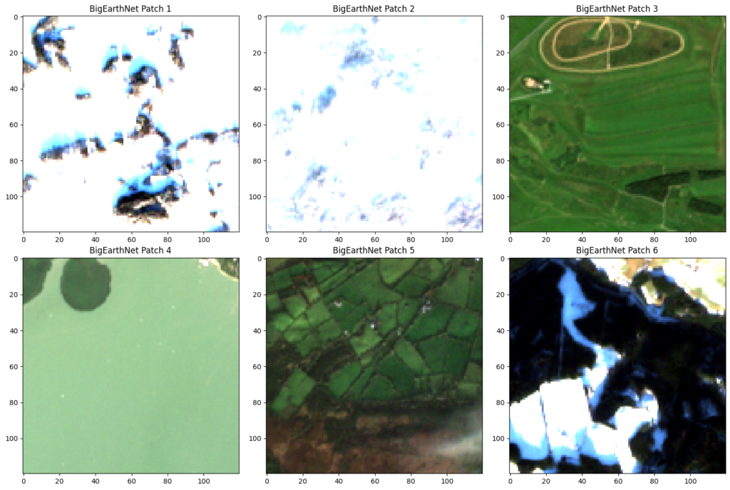
One thing you may notice in the above figure is that some of them look completely fine. For example, patch 3 and 4 look pretty normal, even patch 5 has very minimal cloud coverage. I don’t know how they decided whether something was too snowy or cloudy, but if we eliminate all of the patches that they suggest we end up getting rid of just under 71,000. But, we are still left with ~520,000 patches to train and test with, which is plenty. Furthermore, if we are really in need of more data we can also process the data to get many more patches. Things like rotating the image can instantly give us three more instances of each patch (one per rotation of a patch).
Below I’ve coded a custom data loader which sorts through the snowy and cloudy files and stacks the RGB files together with the label to make them easily accessible for when we bring them into TF and Keras.
import os
import numpy as np
from PIL import Image
import json

def custom_data_loader(data_dir, batch_size, clouds_snow):
    counter = 0
    while True:
        # Initialize empty lists to store images and labels
        batch_data = [[], []]
        num_samples = 0

        # Iterate through subdirectories within the data directory
        for subdir in os.listdir(data_dir):
            # Checks to make sure the cloudy and snowy patches are not included.
            # Since they're ordered we can increment the clouds_snow list one at a time
            if subdir == clouds_snow[count]:
                counter += 1
                continue
            subdir_path = os.path.join(data_dir, subdir)
            if os.path.isdir(subdir_path):
                # Select only files representing RGB spectral inputs (e.g., 'B02.tif', 'B03.tif', 'B04.tif')
                rgb_files = [f for f in os.listdir(subdir_path) if f.endswith(('B02.tif', 'B03.tif', 'B04.tif'))]
                json_path = os.path.join(subdir_path, subdir + '_labels_metadata.json')

                # Load and combine spectra
                rgb_images = []
                for filename in rgb_files:
                    image_path = os.path.join(subdir_path, filename)
                    with Image.open(image_path) as img:
                        # img = img.resize((224, 224))  # Resize image to a common size
                        rgb_images.append(np.array(img))

                combo_image = np.stack(rgb_images, axis=-1)

                # Load labels from JSON file
                json_labels = []
                with open(json_path) as json_file:
                    json_data = json.load(json_file)
                    json_labels = json_data['labels']

                # print(num_samples)
                batch_data[0].append(combo_image)
                batch_data[1].append(json_labels)
                # entry = []
                num_samples += 1

                # Yield batch if batch size is reached
                if num_samples == batch_size:
                    batch_data.append(num_samples)
                    yield batch_data
                    batch_data = [[],[]]

        # Yield remaining images as the last batch
        if images:
            batch_data.append(num_samples)
            yield batch_data
In the code above I parse through the folders (given the root folder directory) and subsequently go through each one and pick out the RGB values. I’m just starting out with the RGB vectors because that nearly quarters the amount of data we have to go through. This is where we’re going to leave off for now, but a part two will be coming very soon, and we will look at how just using RGB compares against using more spectral outputs!
Resources
Data:
https://bigearth.net/#downloads
Research Paper:
G. Sumbul, A. d. Wall, T. Kreuziger, F. Marcelino, H. Costa, P. Benevides, M. Caetano, B. Demir, V. Markl, “BigEarthNet-MM: A Large Scale Multi-Modal Multi-Label Benchmark Archive for Remote Sensing Image Classification and Retrieval“, IEEE Geoscience and Remote Sensing Magazine, 2021, doi: 10.1109/MGRS.2021.3089174.
Additional Resources:
https://docs.kai-tub.tech/ben-docs/index.html
https://keras.io/guides/
https://www.tensorflow.org/tutorials/images/classification
https://machinelearningmastery.com/how-to-develop-a-cnn-from-scratch-for-cifar-10-photo-classification/
- https://docs.kai-tub.tech/ben-docs/labels.html ↩︎
- https://docs.kai-tub.tech/ben-docs/data-source.html ↩︎
Leave a Reply